Find Batch-biased SVGs
Kinnary Shah
Department of Biostatistics, Johns Hopkins Universitykinnaryshahh@gmail.com
Christine Hou
Department of Biostatistics, Johns Hopkins Universitychris2018hou@gmail.com Source:
vignettes/spe.Rmd
spe.RmdIntroduction
A standard task in the analysis of spatially resolved transcriptomics
(SRT) data is to identify spatially variable genes (SVGs). This is most
commonly done within one tissue section at a time because the spatial
relationships between the tissue sections are typically unknown. One
challenge is how to identify and remove SVGs that are associated with a
known bias or technical artifact, such as the slide or capture area,
which can lead to poor performance in downstream analyses, such as
spatial domain detection. Here, we introduce BatchSVG, a
tool to identify biased features associated with batch effect(s)
(e.g. sample, slide, and sex) in a set of SVGs. Our approach compares
the rank of per-gene deviance under a binomial model (i) with and (ii)
without including a covariate in the model that is associated with the
known bias or technical artifact. If the rank of a feature changes
significantly between these, then we infer that this gene is likely
associated with the bias or technical artifact and should be removed
from the downstream analysis. The package is compatible with SpatialExperiment
objects.
Installation
if (!requireNamespace("BiocManager")) {
    install.packages("BiocManager")
}
BiocManager::install("BatchSVG")
To install the development version from GitHub instead:
remotes::install("christinehou11/BatchSVG")Biased Feature Identification
In this section, we will demonstrate the workflow for using
BatchSVG and show how the method helps to detect and
visualize batch-biased SVGs. We will use an SRT dataset from the WeberDivechaLCdata
package.
spe <- WeberDivechaLCdata_Visium()
spe
class: SpatialExperiment
dim: 23728 20380
metadata(0):
assays(2): counts logcounts
rownames(23728): ENSG00000238009 ENSG00000241860 ... ENSG00000278817
  ENSG00000277196
rowData names(6): source type ... gene_name gene_type
colnames(20380): Br6522_LC_1_round1_AAACAAGTATCTCCCA-1
  Br6522_LC_1_round1_AAACACCAATAACTGC-1 ...
  Br8153_LC_round3_TTGTTTGTATTACACG-1
  Br8153_LC_round3_TTGTTTGTGTAAATTC-1
colData names(20): sample_id donor_id ... discard sizeFactor
reducedDimNames(0):
mainExpName: NULL
altExpNames(0):
spatialCoords names(2) : pxl_col_in_fullres pxl_row_in_fullres
imgData names(4): sample_id image_id data scaleFactor
We will use an SVG set that was previously generated using the nnSVG package.
svgs <- read.csv("svgs_LC.csv", check.names = FALSE)Perform Feature Selection using featureSelect()
This function performs feature selection on a chosen subset of SRT data (input) using a predefined set of SVGs (VGs).
To assess the impact of the batch variable in the SRT data, we fit a binomial model per gene (i) with and (ii) without including a covariate in the model that is associated with the batch effect or unwanted variation. Using this model output, we define and as the residual deviance for gene using a binomial model with and without the batch effect, respectively. We calculate a per-gene relative change in deviance (RCD) as . Generally, a higher per-gene deviance suggests that the gene’s expression is more likely to be biologically meaningful. Therefore, a reduction in deviance after accounting for the batch covariate indicates that the batch explains a portion of the variation in gene expression that was previously attributed to biological differences.
In addition to the residual deviance itself, we also consider the ranks of the residual deviances where top-ranked genes have the largest residual deviance and are considered more important. Here, an increase in rank (e.g. from a rank of 1 to a rank of 500) when including the batch variable indicates that the relative importance of the feature is diminished once the batch variable is accounted for. Therefore, in addition to RCD, we also evaluated the rank deviance (RD), which is defined as , where and are the per-gene rank when the binomial deviance model is run with and without the batch variable, respectively.
The featureSelect() function enables feature selection
while accounting for multiple batch effects. It returns a
list of data frames, where each batch effect is
associated with a corresponding data frame containing key results,
including:
Relative change in deviance before and after batch effect adjustment (RCD)
Rank differences before and after batch effect adjustment (RD)
Number of standard deviations (nSD) for both relative change in deviance and rank difference
We use apply featureSelect() to the example dataset
while adjusting for the batch effect of sample_id.
list_batch_df <- featureSelect(input = spe,
    batch_effect = "sample_id", VGs = svgs$gene_id)
Running feature selection with batch...
Batch Effect: sample_id
Running feature selection without batch...
Calculating deviance and rank difference...
list_batch_df <- featureSelect(input = spe,
batch_effect = "sample_id", VGs = svgs$gene_id, verbose = FALSE)head(list_batch_df$sample_id)
gene_id gene_name dev_default rank_default dev_sample_id
1 ENSG00000188976 NOC2L 3887.944 3652 3876.663
2 ENSG00000188290 HES4 6072.325 2060 6002.105
3 ENSG00000187608 ISG15 6148.214 2016 5375.132
4 ENSG00000078808 SDF4 6197.494 1989 6174.812
5 ENSG00000131584 ACAP3 4072.886 3567 4050.140
6 ENSG00000107404 DVL1 4934.273 2925 4905.259
rank_sample_id d_diff nSD_dev_sample_id r_diff nSD_rank_sample_id
1 3619 0.002909944 -0.4134735 -33 -0.4564835
2 2030 0.011699089 -0.3080473 -30 -0.4149850
3 2461 0.143825761 1.2768180 445 6.1556106
4 1914 0.003673372 -0.4043162 -75 -1.0374625
5 3518 0.005615986 -0.3810144 -49 -0.6778088
6 2864 0.005914856 -0.3774295 -61 -0.8438028Visualize SVG Selection Using svg_nSD()
The svg_nSD() function generates visualizations to
assess the impact of the batch variable(s) on the SVGs. It produces bar
charts of the distribution of SVGs based on relative change in deviance
and rank difference, with colors representing different nSD intervals.
Additionally, the scatterplots compare deviance and rank values with and
without batch effects. Using these plots, we can determine appropriate
nSD thresholds for filtering batch-biased SVGs.
The SVGs in red and very far off the line are most likely to be batch-biased SVGs since their deviance and/or rank values are more changed compared to the other SVGs.
plots <- svg_nSD(list_batch_df = list_batch_df,
            sd_interval_dev = 5, sd_interval_rank = 5)
Figure 1. Visualizations of nSD_dev and nSD_rank threshold selection
plots$sample_id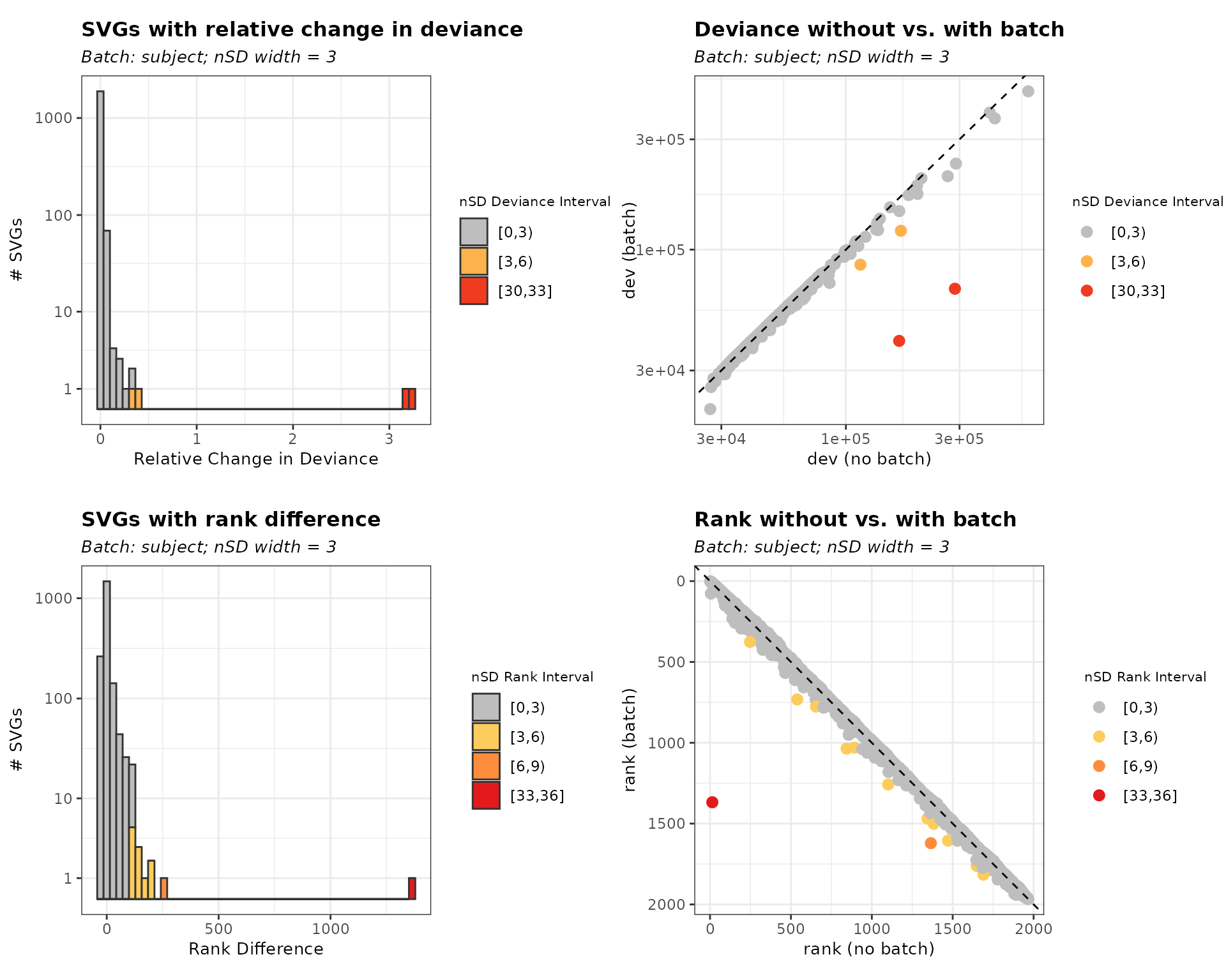
Identify Biased Genes Using biasDetect()
The function biasDetect() is designed to identify and
filter out batch-biased SVGs across different batch effects. Using
threshold values selected from the visualization results generated by
svg_nSD(), this function detects outliers that exceed a
specified number of standard deviation (nSD) threshold in either
relative change in deviance, rank difference, or both.
The function outputs visualizations comparing deviance and rank values with and without batch effects. Genes with high deviations, highlighted in color, are identified as potentially biased and can be excluded based on the selected nSD thresholds.
The function offers flexibility in customizing plot aesthetics, allowing users to adjust the point size (plot_point_size), shape (plot_point_shape), annotated text size (plot_text_size), and color palette (plot_palette). Default values are provided for these parameters if not specified. Users should refer to the ggplot2 aesthetic guidelines to ensure appropriate values are assigned for each parameter.
We will use nSD_dev = 10 and nSD_rank = 8
for the example. Users should adjust these values based on their
datasets. We also include a brief sensitivity analysis below,
visualizing how the number of identified batch-biased genes varies
across a range of nSD values. We have chosen relatively high thresholds
in this example to be more conservative with the SVGs we will filter out
of the SVG list.
vec_dev <- list_batch_df$sample_id$nSD_dev_sample_id[list_batch_df$sample_id$nSD_dev_sample_id > 0]
x_values <- 2:round(max(vec_dev))

counts <- sapply(x_values, function(x) sum(vec_dev > x))

df <- data.frame(
  threshold = x_values,
  count = counts
)

p1 <- ggplot(df, aes(x = threshold, y = count)) +
  geom_point(color = "blue", size = 2) +
  labs(x = "Threshold Value",
       y = "Number of SVGs > Threshold",
       title = "Relative Change in Deviance") +
  theme_minimal()

vec_rank <- list_batch_df$sample_id$nSD_rank_sample_id[list_batch_df$sample_id$nSD_rank_sample_id > 0]
x_values <- 2:round(max(vec_rank))

counts <- sapply(x_values, function(x) sum(vec_rank > x))

df <- data.frame(
  threshold = x_values,
  count = counts
)

p2 <- ggplot(df, aes(x = threshold, y = count)) +
  geom_point(color = "blue", size = 2) +
  labs(x = "Threshold Value",
       y = "Number of SVGs > Threshold",
       title = "Rank Difference") +
  theme_minimal()

plot_grid(p1,p2)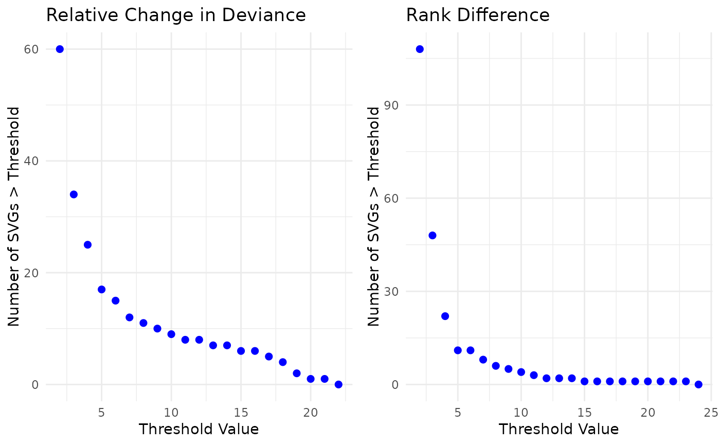
Usage of Different Threshold Options
-
threshold = "dev": Filters batch-biased SVGs based only on the relative change in deviance. Genes with deviance changes exceeding the specifiednSD_devthreshold are identified as batch-biased and can be removed.
bias_dev <- biasDetect(list_batch_df = list_batch_df,
    threshold = "dev", nSD_dev = 10)
Table 1. Outlier Genes defined by nSD_dev only
head(bias_dev$sample_id$Table)
          gene_id gene_name dev_default rank_default dev_sample_id
1 ENSG00000164241   C5orf63    39655.17           16      20707.20
2 ENSG00000198888    MT-ND1   218960.47            3      87994.48
3 ENSG00000198804    MT-CO1   214336.22            5      83576.35
4 ENSG00000198712    MT-CO2   223708.64            2      78899.48
5 ENSG00000198899   MT-ATP6   215486.64            4      81755.33
6 ENSG00000198938    MT-CO3   260433.30            1     100030.36
  rank_sample_id    d_diff nSD_dev_sample_id r_diff nSD_rank_sample_id
1             57 0.9150424          10.52760     41         0.56714614
2              4 1.4883431          17.40436      1         0.01383283
3              5 1.5645560          18.31854      0         0.00000000
4              7 1.8353625          21.56688      5         0.06916416
5              6 1.6357505          19.17252      2         0.02766567
6              3 1.6035425          18.78619      2         0.02766567
  nSD_bin_dev dev_outlier
1     [10,20)        TRUE
2     [10,20)        TRUE
3     [10,20)        TRUE
4     [20,30]        TRUE
5     [10,20)        TRUE
6     [10,20)        TRUE
We can change point size using plot_point_size.
# size default = 3
bias_dev_size <- biasDetect(list_batch_df = list_batch_df,
    threshold = "dev", nSD_dev = 10, plot_point_size = 4)
Figure 2. Customize point size
plot_grid(bias_dev$sample_id$Plot, bias_dev_size$sample_id$Plot)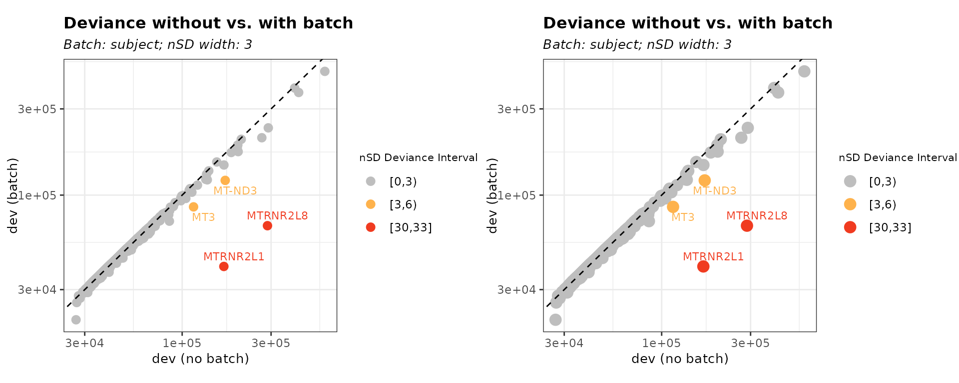
-
threshold = "rank": Identifies biased genes based only on rank difference. Genes with rank shifts exceedingnSD_rankare considered batch-biased.
bias_rank <- biasDetect(list_batch_df = list_batch_df,
    threshold = "rank", nSD_rank = 8)
Table 2. Outlier Genes defined by nSD_rank only
head(bias_rank$sample_id$Table)
          gene_id gene_name dev_default rank_default dev_sample_id
1 ENSG00000173372      C1QA    5524.224         2429      4531.851
2 ENSG00000173369      C1QB    8344.491         1046      5922.112
3 ENSG00000162511    LAPTM5    6101.099         2040      5159.188
4 ENSG00000270188 MTRNR2L11    7880.694         1182      5976.601
5 ENSG00000196136  SERPINA3    6616.945         1753      4130.295
6 ENSG00000105519      CAPS   10670.300          600      7356.179
  rank_sample_id    d_diff nSD_dev_sample_id r_diff nSD_rank_sample_id
1           3198 0.2189775          2.178266    769          10.637448
2           2087 0.4090398          4.458072   1041          14.399979
3           2653 0.1825696          1.741552    613           8.479526
4           2047 0.3185914          3.373140    865          11.965400
5           3469 0.6020515          6.773256   1716          23.737141
6           1307 0.4505222          4.955655    707           9.779813
  nSD_bin_rank rank_outlier
1       [8,16)         TRUE
2       [8,16)         TRUE
3       [8,16)         TRUE
4       [8,16)         TRUE
5      [16,24]         TRUE
6       [8,16)         TRUE
We can change point shape using plot_point_shape.
Figure 3. Customize point shape
# shape default = 16
bias_rank_shape <- biasDetect(list_batch_df = list_batch_df,
    threshold = "rank", nSD_rank = 8, plot_point_shape = 2)

plot_grid(bias_rank$sample_id$Plot, bias_rank_shape$sample_id$Plot)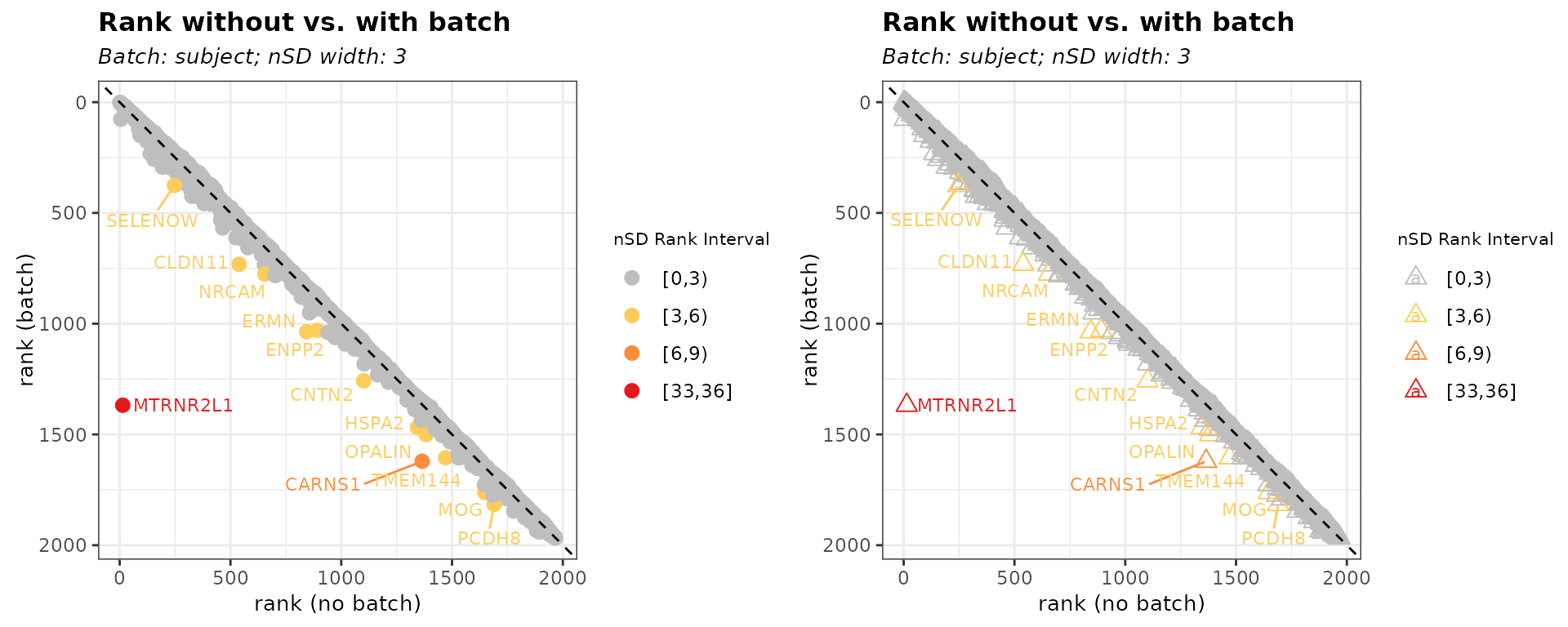
-
threshold = "both": Detects biased genes based on both relative change in deviance and rank difference, providing a more stringent filtering approach.
bias_both <- biasDetect(list_batch_df = list_batch_df, threshold = "both",
    nSD_dev = 10, nSD_rank = 8)
Table 3. Outlier Genes defined by nSD_dev and nSD_rank
head(bias_both$sample_id$Table)
          gene_id gene_name dev_default rank_default dev_sample_id
1 ENSG00000173372      C1QA    5524.224         2429      4531.851
2 ENSG00000173369      C1QB    8344.491         1046      5922.112
3 ENSG00000162511    LAPTM5    6101.099         2040      5159.188
4 ENSG00000270188 MTRNR2L11    7880.694         1182      5976.601
5 ENSG00000164241   C5orf63   39655.169           16     20707.201
6 ENSG00000196136  SERPINA3    6616.945         1753      4130.295
  rank_sample_id    d_diff nSD_dev_sample_id r_diff nSD_rank_sample_id
1           3198 0.2189775          2.178266    769         10.6374484
2           2087 0.4090398          4.458072   1041         14.3999789
3           2653 0.1825696          1.741552    613          8.4795265
4           2047 0.3185914          3.373140    865         11.9654003
5             57 0.9150424         10.527596     41          0.5671461
6           3469 0.6020515          6.773256   1716         23.7371410
  nSD_bin_dev dev_outlier nSD_bin_rank rank_outlier
1      [0,10)       FALSE       [8,16)         TRUE
2      [0,10)       FALSE       [8,16)         TRUE
3      [0,10)       FALSE       [8,16)         TRUE
4      [0,10)       FALSE       [8,16)         TRUE
5     [10,20)        TRUE        [0,8)        FALSE
6      [0,10)       FALSE      [16,24]         TRUE
We can change point color using plot_palette. The
color palette here
can be referenced as the function uses RColorBrewer to
generate colors.
Figure 4. Customize the palette color
# color default = "YlOrRd"
bias_both_color <- biasDetect(list_batch_df = list_batch_df,
    threshold = "both", nSD_dev = 10, nSD_rank = 8, plot_palette = "Greens")

plot_grid(bias_both$sample_id$Plot, bias_both_color$sample_id$Plot,nrow = 2)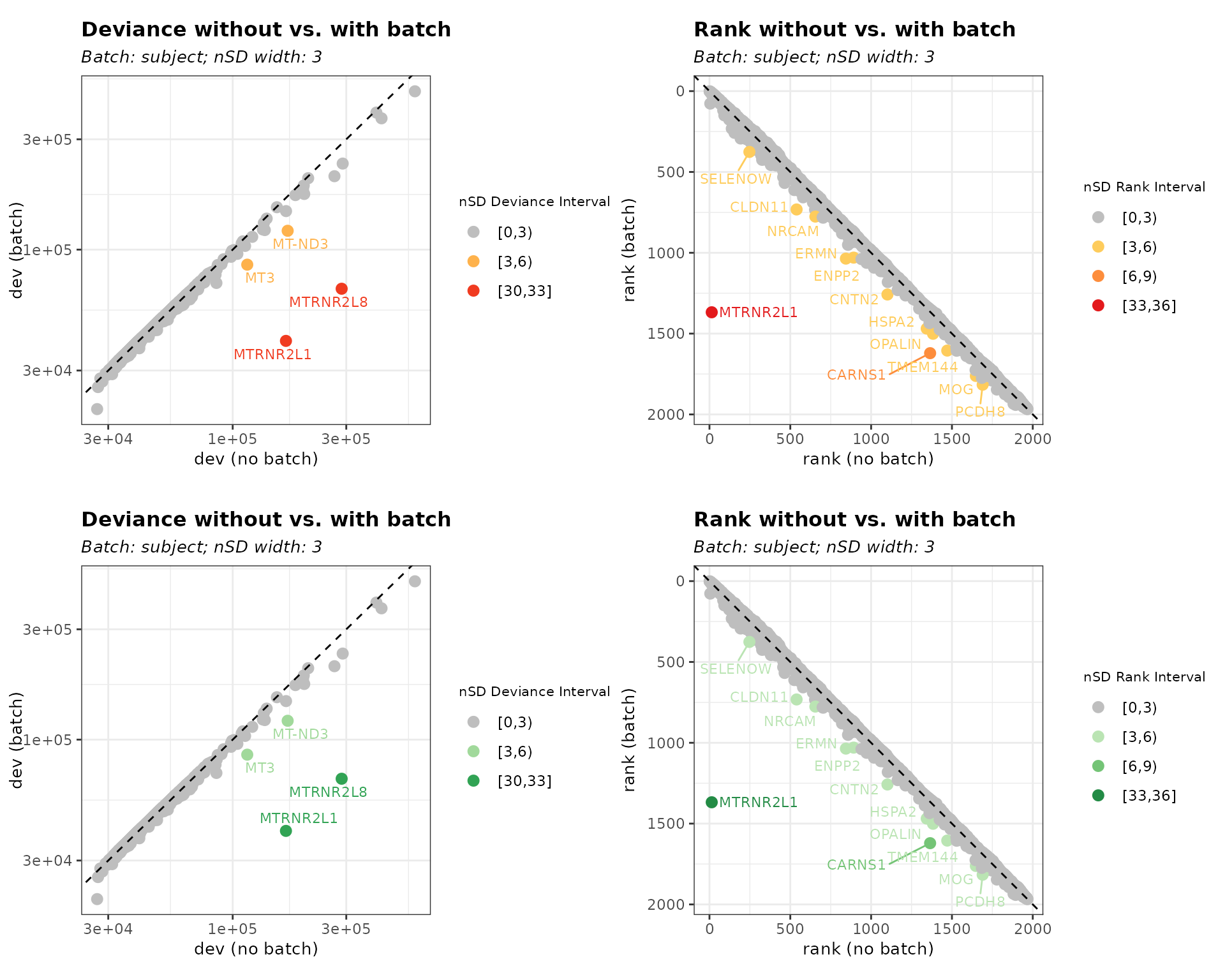
We can change text size using plot_text_size. We can also specify unique color palettes for both batch effects.
Figure 5. Customize text size and color palette
# text size default = 3
bias_both_color_text <- biasDetect(list_batch_df = list_batch_df,
    threshold = "both", nSD_dev = 10, nSD_rank = 8,
    plot_palette = c("Blues"), plot_text_size = 4)

plot_grid(bias_both$sample_id$Plot, bias_both_color_text$sample_id$Plot,nrow = 2)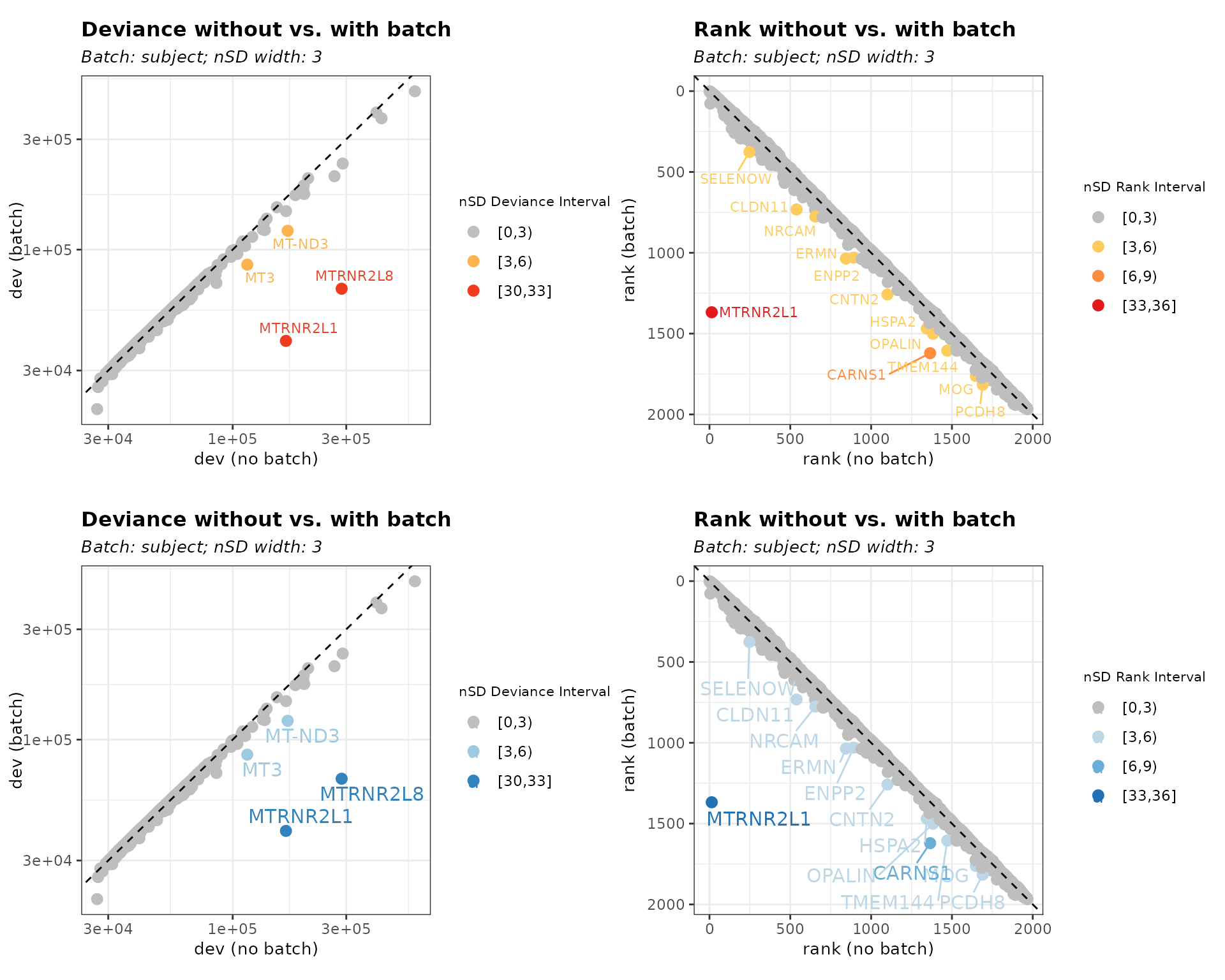
Refine SVGs by Removing Batch-Affected Outliers
Finally, we obtain a refined set of SVGs by removing the batch-biased
SVGs based on user-defined thresholds for nSD_dev and
nSD_rank.
Here, we use the results from bias_both, which applied
threshold = "both" to account for both deviance and rank
differences.
bias_both_df <- bias_both$sample_id$Table
svgs_filt <- setdiff(svgs$gene_id, bias_both_df$gene_id)
svgs_filt_spe <- svgs[svgs$gene_id %in% svgs_filt, ]
nrow(svgs_filt_spe)
[1] 3890
After obtaining the refined set of SVGs, these genes can be further analyzed using established SRT clustering algorithms to explore tissue layers and spatial organization.
R session information
## Session info
sessionInfo()
#> R version 4.6.0 (2026-04-24)
#> Platform: x86_64-pc-linux-gnu
#> Running under: Ubuntu 24.04.4 LTS
#>
#> Matrix products: default
#> BLAS:   /usr/lib/x86_64-linux-gnu/openblas-pthread/libblas.so.3
#> LAPACK: /usr/lib/x86_64-linux-gnu/openblas-pthread/libopenblasp-r0.3.26.so;  LAPACK version 3.12.0
#>
#> locale:
#>  [1] LC_CTYPE=C.UTF-8       LC_NUMERIC=C           LC_TIME=C.UTF-8
#>  [4] LC_COLLATE=C.UTF-8     LC_MONETARY=C.UTF-8    LC_MESSAGES=C.UTF-8
#>  [7] LC_PAPER=C.UTF-8       LC_NAME=C              LC_ADDRESS=C
#> [10] LC_TELEPHONE=C         LC_MEASUREMENT=C.UTF-8 LC_IDENTIFICATION=C
#>
#> time zone: UTC
#> tzcode source: system (glibc)
#>
#> attached base packages:
#> [1] stats4    stats     graphics  grDevices utils     datasets  methods
#> [8] base
#>
#> other attached packages:
#>  [1] ggplot2_4.0.3               cowplot_1.2.0
#>  [3] WeberDivechaLCdata_1.14.0   SpatialExperiment_1.22.0
#>  [5] SingleCellExperiment_1.34.0 SummarizedExperiment_1.42.0
#>  [7] Biobase_2.72.0              GenomicRanges_1.64.0
#>  [9] Seqinfo_1.2.0               IRanges_2.46.0
#> [11] S4Vectors_0.50.1            MatrixGenerics_1.24.0
#> [13] matrixStats_1.5.0           ExperimentHub_3.2.0
#> [15] AnnotationHub_4.2.0         BiocFileCache_3.2.0
#> [17] dbplyr_2.5.2                BiocGenerics_0.58.1
#> [19] generics_0.1.4              BatchSVG_1.5.3
#> [21] BiocStyle_2.40.0
#>
#> loaded via a namespace (and not attached):
#>  [1] tidyselect_1.2.1     dplyr_1.2.1          farver_2.1.2
#>  [4] blob_1.3.0           Biostrings_2.80.1    filelock_1.0.3
#>  [7] S7_0.2.2             fastmap_1.2.0        digest_0.6.39
#> [10] rsvd_1.0.5           lifecycle_1.0.5      KEGGREST_1.52.0
#> [13] RSQLite_3.53.1       magrittr_2.0.5       compiler_4.6.0
#> [16] rlang_1.2.0          sass_0.4.10          tools_4.6.0
#> [19] yaml_2.3.12          knitr_1.51           labeling_0.4.3
#> [22] S4Arrays_1.12.0      htmlwidgets_1.6.4    bit_4.6.0
#> [25] curl_7.1.0           DelayedArray_0.38.2  RColorBrewer_1.1-3
#> [28] abind_1.4-8          BiocParallel_1.46.0  purrr_1.2.2
#> [31] withr_3.0.2          desc_1.4.3           grid_4.6.0
#> [34] beachmat_2.28.0      scales_1.4.0         cli_3.6.6
#> [37] crayon_1.5.3         rmarkdown_2.31       ragg_1.5.2
#> [40] otel_0.2.0           rjson_0.2.23         httr_1.4.8
#> [43] DBI_1.3.0            cachem_1.1.0         parallel_4.6.0
#> [46] AnnotationDbi_1.74.0 BiocManager_1.30.27  XVector_0.52.0
#> [49] vctrs_0.7.3          Matrix_1.7-5         jsonlite_2.0.0
#> [52] bookdown_0.46        BiocSingular_1.28.0  bit64_4.8.2
#> [55] ggrepel_0.9.8        scry_1.24.0          irlba_2.3.7
#> [58] magick_2.9.1         systemfonts_1.3.2    jquerylib_0.1.4
#> [61] glue_1.8.1           pkgdown_2.2.0        codetools_0.2-20
#> [64] gtable_0.3.6         BiocVersion_3.23.1   ScaledMatrix_1.20.0
#> [67] tibble_3.3.1         pillar_1.11.1        rappdirs_0.3.4
#> [70] htmltools_0.5.9      R6_2.6.1             httr2_1.2.2
#> [73] textshaping_1.0.5    evaluate_1.0.5       lattice_0.22-9
#> [76] png_0.1-9            memoise_2.0.1        bslib_0.11.0
#> [79] Rcpp_1.1.1-1.1       SparseArray_1.12.2   xfun_0.58
#> [82] fs_2.1.0             pkgconfig_2.0.3